Boundary Conditions
We now need to select some surfaces and prescribe boundary conditions on them. For our cantilever beam we have two. A fixed end and a loaded end. But we have an implicit model of our problem domain, not an explicit description of its surfaces. So how do we specify surfaces on which to apply our boundary conditions?
Surfaces
The first part of this answer is: another implicit body. We will take the intersection of this body with our original domain to define a surface region. This works well most of the time. But defining a surface by another extended body isn’t always enough to select the surface we want. And defining a surface this way also means our intersecting body has the same requirements as any other feature in our problem: our maximum element size must also be smaller than any feature on this intersecting body.
So we find ourselves at a bit of an impasse. We want a very refined, tightly fitting, intersecting body to better capture our surface, but we don’t want to have to keep shrinking our maximum element size or our simulation will become costly.
We need an additional description of the surface. We’ll call it a directional constraint. If you’re familiar with nTop’s Boundary by Flood Fill method then you will find this similar. Except this works in conjunction with the intersecting body to further restrict the surface to areas where the outward normal is within a given angular threshold of some unit normal vector. With the ability to select a surface by both its spatial extent as well as its local orientation we are in a much better position to define our boundary conditions.
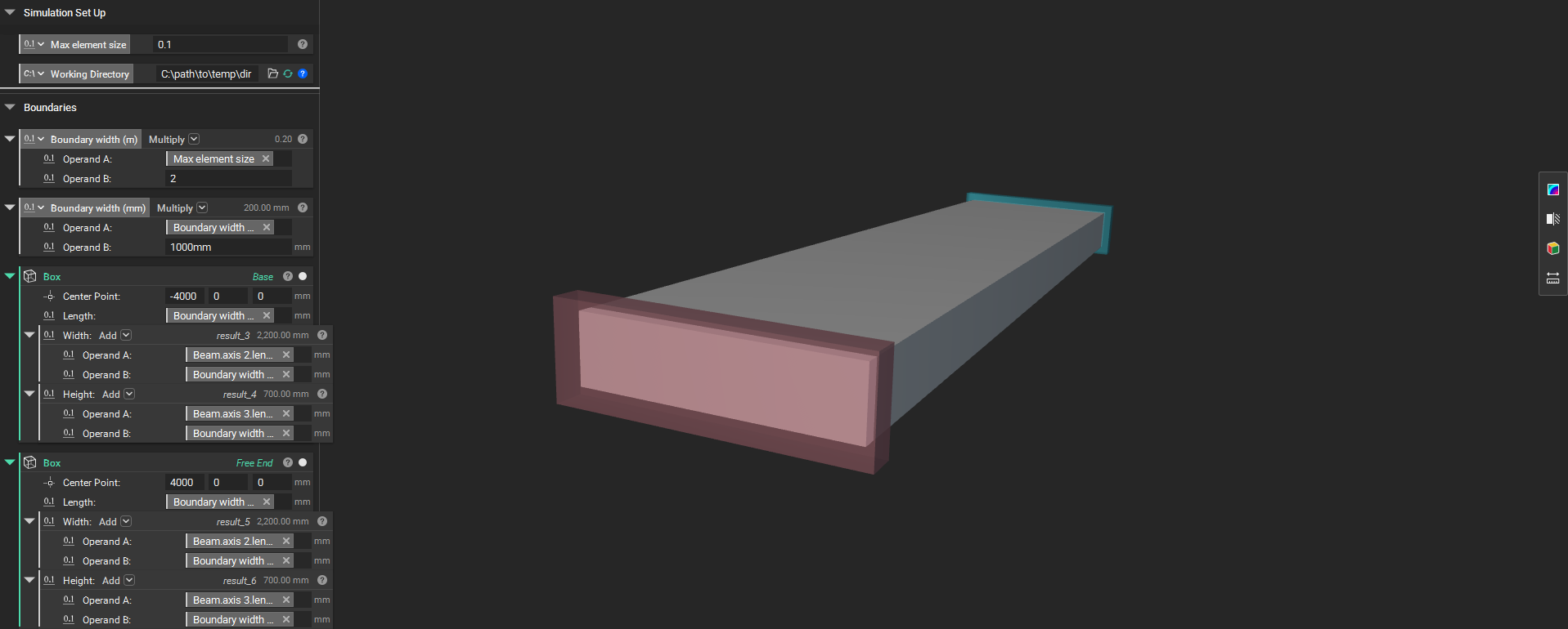
Let’s see how this looks for our beam. We can again use a simple box on each end. But this box will be very thin, and this dimension must be larger than our maximum element size. So we’ll define a boundary box length of twice our maximum element size. We’ll also extend the other dimensions of our bounding boxes by a similar amount since capturing more empty space won’t matter and we want to make sure we don’t miss any edges of our domain.
Note
Multiple boundary conditions accumulate. Care should be taken to ensure that separate intersecting bodies used to effect a common boundary condition do not overlap.
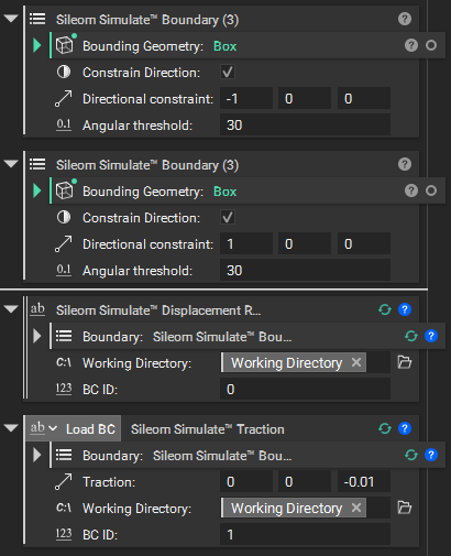
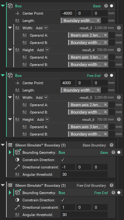
With our intersecting bodies we can now refine the precise surfaces we want to use for our boundary conditions. For our fixed end we’re only interested in the surface whose outward normal points along the negative-x axis. And for the free end we only want the surface whose normal points down the positive-x axis. We’re now going to use our first Sileom Simulate block, the Sileom Simulate Boundary block. Go ahead and select it from the dropdown from our connector blocks. Fill in the parameters as follows:
Bounding Geometry: The box which intersects the fixed end of our beam.
Constrain Direction: Select this box.
Directional Constraint: [-1, 0, 0]
Angular Threshold: We don’t need much of a threshold to capture a flat surface, so let’s just use 30 degrees.
And do the same for the free end:
Bounding Geometry: The box which intersects the free end.
Constrain Direction: Select this box.
Directional Constraint: [1, 0, 0]
Angular Threshold: 30
Conditions
With our surfaces defined we can now set the conditions for our simulation. The fixed end will use a Sileom Simulate Displacement Restraint block. Let’s take a look at the inputs to this block. First we have a parameter for the working directory we set up earlier. This is the first block which will possibly require temporary file access. Then we have a single non-negative integer value which identifies this particular boundary condition. Each boundary condition requires a unique identifier across the notebook.
For the free end we will use a Sileom Simulate Traction block. Bring this block down into the notebook. As with the displacement restraint, the first parameter is the boundary surface. Use the free end boundary we just defined. Second is the applied stress along this surface, in units of N/(m^2). Let’s apply a traction pulling the end downward, [0, 0, -0.01]. The final two parameters are the same as for the displacement restraint block; a working directory and a unique ID.
Note
Each boundary condition’s ID must be unique across the notebook.